|
MAIN PAGE
> Back to contents
Theoretical and Applied Economics
Reference:
Zaytsev M.G., Varyukhin S.E.
Comparison of various methods of assessing the systematic risk factor
// Theoretical and Applied Economics.
2019. № 1.
P. 1-19.
DOI: 10.25136/2409-8647.2019.1.28598.2 URL: https://en.nbpublish.com/library_read_article.php?id=28598
Comparison of various methods of assessing the systematic risk factor
Zaytsev Mikhail Grigor'evich
PhD in Physics and Mathematics
Deputy Director, the Institute of Business and Business Administration, Russian Presidential Academy of National Economy and Public Administration under the President of the Russian Federation
119571, Russia, g. Moscow, pr. Vernadskogo, 82, of. 219

|
mzaytsev08@ibs-m.ru
|
|
 |
|
Varyukhin Sergei Evgen'evich
PhD in Physics and Mathematics
Docent, the Institute of Business and Business Administration, Russian Presidential Academy of National Economy and Public Administration under the President of the Russian Federation
119571, Russia, g. Moscow, pr. Vernadskogo, 82, of. 219
|
|
s.varyukhin63@mail.ru
|
|
|
|
DOI: 10.25136/2409-8647.2019.1.28598.2
Received:
08-01-2019
Published:
08-02-2019
Abstract:
The subject of this research is the calculation of systematic beta risk coefficients for the United States corporations, which in accordance with the A. Damodaran’s industry classification comprise the following branches: Utilities (General), Retail (Grocery and Food), Shoe, Auto&Truck, and Food Wholesalers, with the use of various techniques applied by the famous providers: Yahoo.com, NASDAQ.com, Valueline.com, Bloomberg Terminal, and Damodaran Online. The goal of this work consists in verification and comparison of calculations of the systematic beta risk coefficients for the indicated United States corporations and the substantiation of the revisions to them. The authors calculated the beta coefficients, using the revenue data of these corporation and indexed S&P500, SP500TR, and NYSE Composite; as well as time dependency of beta based on various methods of the famous providers for 43 of the oldest and most sustainable corporations in the United States. The scientific novelty is defined by the fact that the calculations conducted by the authors in accordance with various techniques for the corporations rated on the market NYSE and NASDAQ, practically align with the data of the listed providers, but drastically differ for the diverse assessment techniques applies thereof. For the branches Utilities (General) and Retail (Grocery and Food), the authors’ results for industry beta, calculated as weighted average for the industry with the weights equal to capitalization of corporations, practically coincided with the data of Damodaran Online. However, for the tree other verified industries, the author detected significant, inexplicable discrepancies, clearly related to the presence of small companies in the list of industry, which stocks are irregularly traded in over-the-counter markets.
Keywords:
systematic risk factor, beta coefficient, cost of equity, risk coefficient estimation, Damodaran classification, USA companies, Utilities industry, Retail industry, Internet Providers Techniques, Food Wholesalers industry
Introduction
The assessment of the investment attractiveness of a project or the market value of a company, according to classical financial theory [1– 3], is inextricably linked with the assessment of the non-diversified risk that this financial asset contributes to the investor's diversified portfolio. The higher this non-diversified or otherwise systematic risk, the higher the return required by the investor from this asset [4]. According to the portfolio theory [1], the yield of each asset in the portfolio can be represented as
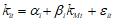 (1) (1)
where all variables with the index t are random, αi – is chosen so that the average value of ε it is zero, and β i is the covariance of the random return of the asset and the market portfolio divided by the variance of the market portfolio σ 2 M
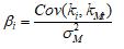 (2) (2)
At the same time, εit characterizes individual characteristics of the asset and does not correlate with the profitability of the market portfolio. Then, the risk of a portfolio composed of n assets with the same weight (assuming that εi and εj are independent variables), expressed by its variance, will be equal to
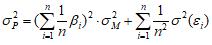 (3) (3)
By entering obvious notation for the average values, we get
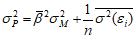 (4) (4)
where the second term tends to zero as the portfolio size increases (i.e. individual asset risks are fully diversified), and the portfolio risk is entirely determined by its covariance with the market portfolio. However, the higher the β i value for the assets that make up the portfolio, the higher the risk of the portfolio. This determines the value of the coefficient β i, as the coefficient of systematic risk of an asset: the higher the value β i, the greater the risk that the asset contributes to this portfolio.
The theory of capital asset pricing (CAPM) [2, 3, 5 –8] relates the required return on a given asset (the required return on equity invested in this asset) to the systematic risk coefficient β:
 (5) (5)
where kRF – risk-free return, and kM– expected return of a market portfolio, which is most often considered a portfolio based on the s&P500 index with shares of companies included in the S &P500 list, proportional to their capitalization.
Although the assumptions of the CAPM theory are subject to reasonable criticism [9], alternative theories provide significantly less opportunities for their empirical verification and predictions [3, 8, 10, 11]. It is important, however, that all researchers agree that compensation in the form of additional returns ("premium" for risk) only deserves an investor who has a well-diversified portfolio, whose risk cannot be more diversified and is determined by macroeconomic conditions. These conditions should be reflected by the yield of the market portfolio, and the risk premium itself - by the systematic risk coefficients of the assets included in the investor's portfolio, in accordance with the formulas (1-4).
The required return on equity is determined by the CAPM theory or another model [12 – 17] this is a matter of empirical research of the documented experience of financial markets. It is important, however, that this "risk premium" should depend on the systematic risk coefficients "beta" i, which determines their exclusive role in financial theory.
However, it is not easy to measure the systematic risk coefficients of certain stocks based on historical data on their profitability. Like many other statistical coefficients, the coefficient β is not stable, neither to deviations from the normal distribution [18 –20], which is exactly the case in the case of market returns and individual shares, nor to the appearance of significant outliers, which is also not uncommon in financial markets)
In the article [21], Damodaran draws attention to the fact that the result of calculating the coefficient β depends not only on which index is selected to represent the market portfolio, and not only on the time period for which data on the yield of this asset and market portfolio are selected (which is more or less natural), but also on what time intervals these returns are fixed. Moreover, if the variation of the coefficient β due to the first two factors does not exceed 10% -15% for the example considered in Damodaran's article with the Walt Disney Company, then the change β due to the change in the choice of time intervals through which returns are fixed can be from 2 to 3 times [21]. This example was used by Damodaran to justify the practical impossibility for an investor to calculate systematic risk coefficients based on the regression of data on the returns of the company of interest and the returns of the market portfolio.
As an alternative, Damodaran offers a so-called "bottom-up" approach to assessing the systematic risk coefficients of various companies or divisions of the company involved in different businesses [8, 21, 22]. The approach is based on the fact that the coefficient β significantly depends not only on what industry the company or its various divisions work in, but also on the financial and operational leverage of the company or division [3, 8, 23].
In order to evaluate the company's or business unit's beta ratio in this case, Damodaran recommends taking from a reliable provider [31] data on the industry average value of the systematic risk ratio, converted to zero debt using the Hamada formula [3, 8] β unlevered, and using this value to calculate the company's (or business unit's) coefficient taking into account financial and operational leverage, and for a complex company consisting of several business units, calculate the βas a weighted average β I its divisions.
At the same time, the reliable provider still calculates the "beta" i of various companies in the industry by regressing data on their returns and market returns with all the problems of such calculation described earlier. Interestingly, despite the clear indication of the ambiguity of such calculations in Damodaran's article [21, 22], this did not force the various "beta" data providers of individual companies or the industry as a whole to somehow coordinate or streamline their calculations.
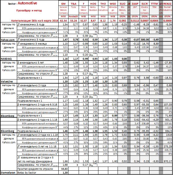
Comparison of systematic risk coefficients calculated by different providers and verification of industry data from Damodaran's website .
The authors checked the coefficients β i of US companies that make up five industries with very different systematic risk coefficients according to the Damodaran classification [31] :
· Utility (General) production and transmission of electricity and gas (industry βlevered =0.29),
· Retail (Grocery and Food) retail food products (industry βlevered =0,71),
· Shoe manufacturing (industry βlevered =0.88),
· Auto&Truck – automotive industry (industry βlevered =1,2),
· Food Wholesalers wholesale trade groceries and related products (industry βlevered =1,79).
The results of the authors ' calculations in comparison with the data of the providers listed above are presented in files on the cloud [30].
Data on the returns of these companies and the returns of the S&P 500, SP500TR and NYSE Composite indices are taken from the open source finance.yahoo.com as of March 2018. Data from various providers about β i companies is obtained from open sources yahoo.com, nasdaq.com, valueline.com, and via Bloomberg Terminal.
At the same time, the site yahoo.com for each of these companies, it gives estimates of βi values based on data on monthly returns over a period of 3 years, using stock rates adj _ close . In this case, it seems logical for the authors to use the SP500TR index (Total Return, which capitalizes the dividends paid by the companies included in the index). However, since the provider does not specify this clearly, the authors estimate beta coefficients based on stock price regressions adj _ close both on the yield of the SP500TR index and on the yield of the standard SP500 index.
Bloomberg Terminal estimates β i based on weekly data for a period of 2 years (using close values for stock prices and the standard s&P 500 index (SPX)), then adjusts the resulting values using the formula
 (6) (6)
justifying this correction by referring to Blum's article [1], which empirically showed that large portfolios with a low or high average value of βP, estimated from monthly returns for 7 years, in the next 7 years demonstrated βP closer to the 1 – average value of the market portfolio beta. As a result, Blum suggested tweaking the β P calculated over the past 7 years using a formula close to (6) in order to predict βP in the next 7 years. Blumberg tweaks the same way β i calculated over the past 2 years from weekly data to predict β i next year (which, of course, is not the same).
Value Line (valueline.com) estimates β i based on weekly data for 5 years, but uses the NYSE Composite portfolio and the yield regression calculated from close values for comparison. Value Line also corrects the βi values using its own formula [24]
 (7) (7)
The Damodaran website States that β i is calculated based on weekly data for 2 years and 5 years (using adj_close stock prices and the SP500TR index), after which a weighted average score is taken with weights of 2/3 and 1/3, respectively.
And finally, on the site nasdaq.com "reliable provider" does not disclose the method of calculating βi, however, the authors found that the βi values close to those issued by this provider can be obtained based on daily data on the returns of close and S&P500 for a period of 3 months.
A comparison of the authors ' calculation results with the data of reliable providers shows that, despite the existing undocumented details of the calculation methods of beta i, there is a good coincidence of results for companies whose shares are regularly traded on the NYSE and NASDAQ stock exchanges. Small differences (much smaller than the 95% confidence intervals defined by the authors for the obtained betas) may be due to the fact that the beta coefficient values were obtained by the authors and providers on different dates. Since it is not possible to present the results of calculations compactly, the authors of suggest viewing specific calculations directly in files uploaded to the cloud [30].
A different picture is observed for companies trading on OTC OTC (Over the Counter) markets. The data columns for these companies in figure 1-5 are grayed out. These companies are characterized by low (often microscopic) capitalization and irregular trading. Rare OTC sales sometimes lead to«Grand » price changes and give single outbursts of fantastic returns. For example, for Rexhall Industries, Inc. (REXLQ, auto&Truck sector, file Betas_Automotive_2018.xlsm) 27.03.17 year asset price according to Yahoo.com was $0.0002 per share. From 27.03.17, there were no sales at all for six weeks, on 15.05.17 the price of $0.0002 was confirmed, and on 22.05.17 the share price rose fantastically to $0.009, giving a yield of 440% for the week. Then there were no sales for another 10 weeks, and on 31.07.17 the stock fell to $001 after which there were no sales again for another 3 weeks.
A different picture is observed for companies trading on OTC OTC (Over The Counter) markets. These companies are characterized by low (often microscopic) capitalization and irregular trading. Rare OTC sales sometimes lead to«grandiose » price changes and give single outbursts of fantastic returns. For example, for Rexhall Industries, Inc. (REXLQ, auto&Truck sector, file Betas_Automotive_2018.xlsm) 27.03.17 year asset price according to Yahoo.com amounted to $0.0002 per share. From 27.03.17, there were no sales at all for six weeks, on 15.05.17 the price of $0.0002 was confirmed, and on 22.05.17 the share price rose fantastically to $0.009, giving a yield of 440% for the week. Then there were no sales for another 10 weeks, and on 31.07.17 the stock fell to $0.001 after which there were no sales again for another 3 weeks. how do I count the weekly return in this case? If we assume that in the absence of trading, the price of shares does not change, then we must assume that the yield in these 10 weeks was zero, and then was ($0,001-$0,009)/$0,009=-89%. However, it can be argued that this price change occurred in 10 weeks, not one. Maybe then it is more correct to «spread » this jump in returns for 10 weeks?
The authors approach this dilemma radically: if there were no sales of shares in a given week, the share price is undefined (rather than remaining the same). A stock's weekly return can only be calculated when two consecutive weeks of trading have taken place. To calculate the beta coefficient of such companies, it is incorrect to use the standard MS Excel KOVAR functions.In() and DISP.In (), and the linear () function for calculating the regression coefficient. In this case, the authors wrote a special function LinRegRel (..), which calls the standard Excel function =linear(..) ( LinEst (..) ), first removing rows with empty and invalid values from the input arrays that cause the standard function to return an error.
Perhaps this solution is too radical authors, as part of the data in the row of stock prices is discarded (if the trading this week was not preceded by an auction the previous week, or the auction this week was not trading next week). Perhaps because of this decision, the data on the beta coefficient for this company (and in other similar cases) is very different from the data of other providers.
The authors receive for REXLQ on weekly returns for a period of 2 years (as of January 1, 2018) a completely "odious" value of "beta" i=1318 (with a 95% confidence interval of 1101), Bloomberg gives an equally odious value of "beta" i=501 (with a 95% confidence interval of 538). For the same company, but as of March 6, 2018, the authors receive βi=0.68 (with a 95% confidence interval of 26 and a 0% determination coefficient), and when using the ValueLine method, the authors receive βi=-28 (with a 95% confidence interval of 41). None of the providers other than Bloomberg (neither Yahoo, nor NASDAQ, nor Value Line) gives beta for this company.
Such«odious » beta values are rare, but if we talk about small companies trading on OTC markets, the values βi= ±5 ÷7, or even±20 ÷50 – are not uncommon. At the same time, the confidence intervals of beta estimates in these cases are comparable or significantly larger than the estimates themselves, and the coefficients of determination are very small. The latter actually means that the null hypothesis that the beta coefficient does not differ from zero cannot be rejected either when evaluating β =300 or when evaluating β = -50. In addition, we clearly meet here with cases where the statistical definition of the systematic risk coefficient beta becomes meaningless, since this coefficient is determined by one or more colossal "outliers". Thus, it is obviously impossible to include such companies in the assessment of the industry beta βsector. However, Damodaran includes them in the list of companies representing the industry.
The authors support the idea of Damodaran [8, 21] to evaluate the systematic risk coefficients of a company using the "Bottom-Up" method (especially in emerging markets), taking as a starting point the systematic risk coefficient of the sector as a more stable characteristic compared to the "beta" of a particular company, calculated as the average value of the coefficients of the "beta" I companies that are most representative of this industry. However, after reviewing the list of companies that make up the us automotive industry in the Damodaran Betas by Sector table for 2017 [31], the authors were surprised to find that of the 18 companies included in this list, Only 6 have a capitalization of $1.76 Bio to $62.4 Bio and have a more or less stable position on the NYSE and NASDAQ stock markets. The remaining 12 companies are irregularly traded on OTC markets and have small and often microscopic capitalizations (from $12K to $92Mio). ZAP, for example, with a capitalization of about $11Mio (400 employees), had a maximum price per share of $1.89 at the end of 2010, but since then the price per share has fallen steadily and is now $0.01 - $0.02. Yahoo.com gave for this company in 3.05.2017 β=-1.88, and 29.12.2017 β=-0.88. Electric Car Company Inc. with a capitalization of $682K has weekly trading volumes on the OTC market from several thousand to $14 Mio, and the price per share of $0.0001, unchanged since 2011. At the same time, Yahoo calculates for this dig β, which on 3.05.2017 was equal to 289, and on 6.03.2018 was 300 (the authors get -9.29 with a confidence interval of 34.59). Similarly, T3M Inc. has a capitalization of $332K (number of employees 37), and a share price of $0.014, and at the time of the company's formation in the spring of 2010, the shares were worth $9. For this company Yahoo.com gives β=-3.49, of course, without any indication of the standard deviation of such «estimates » (the authors received -3.61, but a 95% confidence interval of 9.32). The company ELIO with a capitalization of $92Mio (the maximum among these exotics, although the number of employees is only 28), has been in existence for just over 3 years. The company's share price at the time of its formation on 22.02.2016 was $40, but it has always been declining and is now $3 per share. Yahoo gives it -3.38, which is close to the value obtained by the authors, but the 95% confidence interval for such an estimate is 3.74. All companies, of course, are unprofitable, with earnings per share less than zero.
Fig. 1. Auto &Track
It is difficult to agree that all this must be taken into account. Perhaps all of these newly emerging companies that produce three-wheel electric cars are the future of the U.S. automotive industry. But to what extent do they characterize the current state of the industry and its industry beta? Why are they on the list of companies that make up the us automotive industry? How to account for all these unprofitable companies with irregular sales in OTC markets? If we take the weighted average values of β i of these companies (with weights equal to the capitalization of the companies), then the 12 exotic companies listed above will not have any impact on the industry βsector. However, Damodaran pointed out in his papers [8, 21] that if the industry is dominated by one or a small number of companies with high capitalization, calculating the weighted average βsector will not significantly reduce the standard deviation of the βsector estimate. Therefore, it is better to consider all β i with the same weight. Then, according to Damodaran, the standard deviation will decrease in  times, where n – is the number of companies in the industry. It is obvious, however, that there will be no reduction in the standard deviation of the average beta rating in this case, since the standard deviations of the beta I ratings of all these 12 exotic companies are huge and far exceed the standard deviations of the beta ratings of normal companies, even if the capitalization of one such company dominates all the others. times, where n – is the number of companies in the industry. It is obvious, however, that there will be no reduction in the standard deviation of the average beta rating in this case, since the standard deviations of the beta I ratings of all these 12 exotic companies are huge and far exceed the standard deviations of the beta ratings of normal companies, even if the capitalization of one such company dominates all the others.
In connection with all the above, the authors are not always able to get the average values of the industry βsector presented in the Betas by Sector tables on the Damodaran website. In the case of Utilities (General) and Retail (Grocery and Food) industries, the industry beta βsector of Damodaran and the weighted average beta for the industry with weights equal to the capitalization of companies calculated by the authors are almost identical. For the Shoe industry, the weighted average beta calculated by the authors with weights equal to the companies ' capitalization is in the 95% confidence interval (0.87; 1.35), and Damodaran gives an estimate that falls on the edge of this interval β sector=0.88. However, for the other two industries studied by the authors, neither the average weighted by the capitalization of companies (which is natural), nor the simple average (mentioned in the book and article by Damodaran [8, 21] according to theβi obtained in our calculations) completely coincide with the data in the Damodaran tables. For the Auto & Truck industry, authors get a weighted average beta in the 95% confidence interval (1.51; 1.85), and Damodaran gives the value of the industry beta βsector=1.20. For the Food Wholesalers industry, the authors ' score is in the 95% confidence interval (0.58; 1.00), and Damodaran gives theβsector=1.79.
What intermediate averaging option has been used by a reliable provider to calculate the industry beta for the Auto&Truck and Food Wholesalers industries in the USA remains a mystery for the authors .
The authors calculate the standard deviation of the weighted average beta industry estimate using an obvious formula
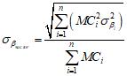 (8) (8)
where is the MCi – market capitalization of the i-th company.
Of course, in this formula, instead of standard deviations, you can immediately substitute 95% confidence intervals, which is done in MS Excel tables presented in files in the cloud [30].
Apparently, the provider of Damodaran's βi coefficients (S&P Capital IQ) does not calculate βi as indicated on the Damodaran site, and the industry βsectors listed in the Damodaran tables undergo some kind of processing not specified on the Damodaran site.
Note that for the Food Wholesalers industry, out of the 15 companies that Damodaran included in the industry list, 8 are the same exotic companies with microscopic capitalization, trading on OTC markets and having abnormal beta values, as well as those considered in detail for the Auto&Truck industry. For example, for PCFP (Cannabis Leaf Inc.), Yahoo gives β=-125, Bloomberg on January 1, 2018 gives β=+102 (with a 95% confidence interval of ±47), and the authors received β=-1.72 (with a 95% confidence interval of ±5.63). In contrast, for the Shoe industry (where our result is closer to The value of the Damodaran industry beta), there are only 4 out of 11 such OTC companies. Similarly for the Retail (Grocery and Food) industry, – only 4 out of 14 companies are traded on OTC markets, and for Utilities (General) – all companies included in the industry are traded on the NYSE and have«decent » beta values and comparable capitalizations. As noted above, for the last two industries, our calculations of industry betas coincide with those presented by Damodaran.
All this raises serious questions about the formation of a list of companies that represent the industry for calculating the industry beta.;
Returning to the comparison of data from various "reliable" providers, it should be emphasized that none of the cited providers, except Bloomberg, indicates either the coefficient of determination of regressions that were evaluated by "beta" i, or the standard deviation of the estimation of these systematic risk coefficients. Meanwhile, the calculations made by the authors show that 95% confidence intervals for β i are very large even for stable companies.
It can be seen that the differences in the estimates of βi stable companies based on the methodology of different providers made by the authors often significantly exceed the 95% confidence intervals obtained by the authors. This may be due to the fact that the assumption of a normal distribution of regression balances does not hold when it comes to returns in financial markets. Many papers [25–29] have pointed out that the distribution of returns of various stocks, the S &P500 index, and other indices is far from normal and is characterized by long "tails", a large number of outliers significantly exceeding 3 Sigma. Then, the statistical error in determining the coefficients of β i will be even greater than indicated by the standard regression procedure.
This raises the question, which of the methods of evaluating β i is more reliable and adequate to the main purpose of determining the industry βsector - the assessment of the required return on equity?
When evaluating the attractiveness of a particular interval between successive moments of fixing the index and the stock price, as well as the period at which the "beta" is evaluated, it is necessary to take into account the following obvious "pros and cons" [8, 21]. Daily fixing of indices and stock prices will obviously give a greater value of points in the sample to determine β on any evaluation period than weekly or monthly data. This, in turn, should lead to greater accuracy of the estimate (less standard deviation of the estimate βi). However, the relative random spread of daily stock prices, measured as a percentage of the average daily return, is obviously higher than in the case of weekly, monthly, and even more so annual intervals. Therefore, it is preferable to take longer intervals to evaluate long-term correlations between the stock price and the market index.
As for the period at which βi is evaluated, from the point of view of a bona fide investor participating in a long-term project, or knowingly investing money in a particular company for a long time, it is desirable to know the average value of βi for a relatively long period of 5–10 years. For the same reason, when evaluating the required return on equity, Damodaran [8] recommends using the risk-free yield of 10-year (rather than 3-month) us Treasury bonds. However, when evaluating β i for a long period in the past, you will have to forecast βi for approximately the same period in the future (although the forecast can be adjusted annually), and over such a long period of time (10– 20 years), not only in an individual company, but also in the industry as a whole, there may be noticeable changes that can significantly affect the systematic risk ratio of the industry.
Therefore, all "reliable providers" tend to take smaller periods for evaluating βi in order to produce more up-to-date» data (Yahoo.com – 3 years, Bloomberg – 2 years, and NASDAQ – 3 months). At the same time, the βi scores tend to change very much from year to year.
Calculating the time dependence of the systematic risk coefficient for 43 companies listed on the markets NYSE and NASDAQ since 1962 – 1970s.
While "reliable providers" tend to take smaller periods for evaluating "beta" i, these " LRM " estimates tend to change very much from year to year.
Thus, Damodaran in [31] gives for the same industry Auto&Truck in different years the following industry β sector (without specifying the standard deviation of the estimate).
Table 1. Industry coefficients β for Auto & Truck ( Automotive ) according to Damodaran's assessment.
|
Years
|
2011
|
2012
|
2013
|
2014
|
2015
|
2016
|
2017
|
|
Industry β for Auto & Truck
|
1,589
|
1,729
|
1,277
|
1,095
|
0,955
|
0,845
|
1,2
|
The question arises whether these changes are a real reflection of changes in macroeconomic factors that affect the systematic risk of the industry, or are they the result of imperfect assessment methods? What happened to the us automotive industry in the 4 years from 2012 to 2016 (data for 5.01.2017, even before trump took office as President of the United States) that, being at first 1.7 times more risky than the market as a whole, it became by 2016 not only less risky than the market, but even less risky than the production of soft drinks (βsector=0.91), the systematic risk of which is traditionally lower than the market?
The authors checked how β i changes over time for 43 old and stable companies listed on the NYSE and NASDAQ stock markets, whose price data is available on Yahoo.com from 1962-1970, if you calculate them for a period of 3 months, 2 years, 5 years and 10 years based on daily prices. Figure 6 (a-d) shows examples of βI (t) dependencies for Boeing Co., Coca-Cola Co., Hewlett-Packard Inc., and Chevron Co., calculated in increments of 21 business days (1 month). On the same charts, we show the average value of the 95% confidence interval for the corresponding estimates β i (files with data and calculations for 43 well-known companies are available in the cloud at the link (https://1drv.ms/f/s!Arfri2i3v3yxjcvdqlhbr1ufuidug, file Beta(t)43comp1962-2018. xlsm. All the features of βi(t) dependencies noted below for different periods are valid for all the companies studied.
Table 2 shows the average and maximum value of the 95% confidence interval for the evaluation of β i different time points in absolute values and as a percentage of the evaluation value.
Table 2. Confidence intervals for estimates of coefficients β for stable companies that have long been listed on the markets NYSE and NASDAQ , for different evaluation periods.
|
|
95% confidence interval ±
|
|
Company
|
Period
|
3 months
|
2 years
|
5 years
|
10 years
|
|
Boeing Co.
|
Average
|
0,53
|
0,17
|
0,11
|
0,07
|
|
Maximum
|
1,98
|
0,38
|
0,19
|
0,13
|
|
Average % of the rating value
|
60%
|
16%
|
9%
|
7%
|
|
Coca-Cola Co.
|
Average
|
0,35
|
0,12
|
0,07
|
0,05
|
|
Maximum
|
1,21
|
0,21
|
0,11
|
0,07
|
|
Average % of the rating value
|
50%
|
15%
|
9%
|
6%
|
|
Hewlett-Packard Inc.
|
Average
|
0,58
|
0,19
|
0,11
|
0,07
|
|
Maximum
|
2,10
|
0,39
|
0,19
|
0,12
|
|
Average % of the rating value
|
85%
|
14%
|
9%
|
6%
|
|
Chevron Co.
|
Average
|
0,36
|
0,12
|
0,07
|
0,05
|
|
Maximum
|
0,83
|
0,18
|
0,10
|
0,07
|
|
Average % of the rating value
|
50%
|
16%
|
9%
|
6%
|
Table 2 and figure 2 (a-d) show that for a 3-month evaluation period, this confidence interval is comparable to, and possibly exceeds, the typical amplitude of frequent spikes and troughs in the βI (t) graph. for Boeing Co., for example, the average value of 95% of theβI confidence interval is 0.53, and the maximum value is 1.98. for all 4 companies, the average value of 95% of the confidence interval as a percentage of the estimated value is I is 50% -85%, and the maximum can be many times higher than the estimate itself. The very "nervous" behavior of the chart β i(t) does not allow us to consider it a real change in the indicator of systematic risk of the company. Is it possible for βI Boeing Co to change from -0.25 to 3, and Coca-Cola – from -0.5 to 2? It is obvious that all these frequent fluctuations with high amplitudes are the result of errors in the estimation of β i.
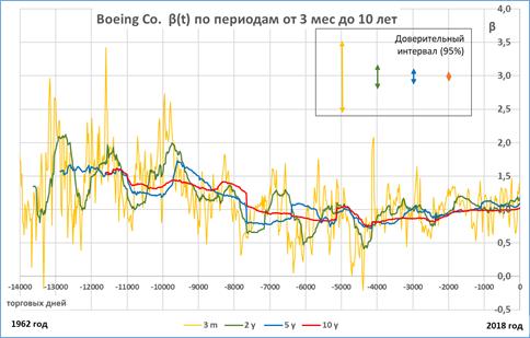
Fig. 2A. The dependence of the ratio β ( t ) for Boeing Co . from 4/01/1962 (-14000 business days from March 2018-the moment the authors processed daily data Yahoo . com ) after every 21 business days (approximately 1 month)
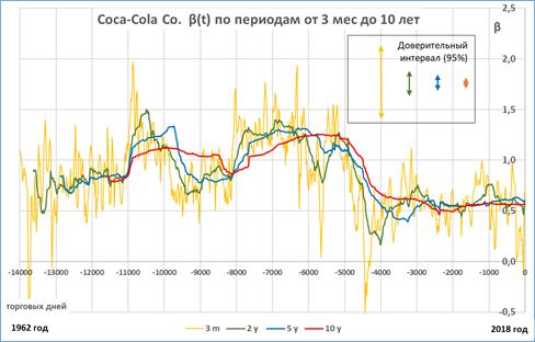
Fig. 2 b . The dependence of the ratio β ( t ) for Coca - Cola Co . from 4/01/1962 (-14000 business days from March 2018-the moment the authors processed daily data Yahoo . com ) with an interval of 21 business days (approximately 1 month)
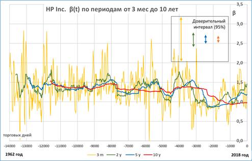
Fig. 2C. The dependence of the ratio β ( t ) for Hewlett - Packard Inc . from 4/01/1962 (-14000 business days from March 2018 — the moment the authors process their daily data Yahoo . com ) with an interval of 21 business days (approximately 1 month)
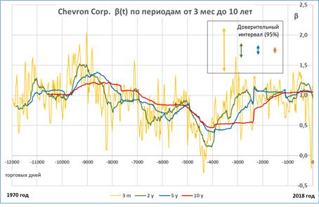
Fig. 2 d . The dependence of the ratio β ( t ) for Chevron Co from 5/01/1970 (-12000 business days from March 2018-the moment the authors process daily data Yahoo . com ) with an interval of 21 business days (approximately 1 month).
For a 2-year period, the typical amplitudes of the humps and depressions of the graph βi (t), although in most cases greater than the average value of 95% of the confidence interval of the estimate βi, is still quite comparable to it. In addition, it is difficult to explain the periodic change in the systematic risk coefficient, for example, for Boeing Co from β=1 to β=2 with an average period of 6 years several times in a row, followed by a wave-like decrease to β=0.5. Or undulating (with a period of 7 to 15 years) change in the coefficient β for Chevron Co from β=1.5 to β=0.15.
However, if we compare these humps and depressions in the βi(t) charts for a two-year period for all companies with a smoother change in βi(t) for 5-year and 10-year periods, then their value is naturally explained by a statistical error in the βi(t) estimation.;
Obviously, using a sample of historical data over a short period to evaluate β i is counterproductive, since most of the observed variations in time β i(t) are simply the result of a statistical error in its estimation. The authors believe that for the purpose of estimating the required return on equity, it is much more useful to have more stable and slowly changing estimates of βi(t) over periods of 5-10 years than erratic and difficult to explain fluctuations of βi (t) with a high frequency and amplitude.
Impact of choosing an index representing a market portfolio
A separate issue is the use of the classic s&P500 index to represent the market portfolio by providers Bloomberg, NASDAQ, and possibly Yahoo. The fact is that if you make a real portfolio based on the s&P500 index, i.e. include in the portfolio shares of companies listed in the S&P500 list, in an amount proportional to the capitalization of the companies, the resulting portfolio will give a different return than the standard s&P500 index, since the latter does not take into account the dividends paid by these companies. This circumstance was noted in [8, 21] when criticizing the Bloomberg calculation method β. Does not accounting for dividend payments by companies in the market portfolio affect the valuation of β?
To answer this question, the authors calculated the βi coefficients for the same 43 companies on several dates in the past, comparing Adjusted Close for these companies with the SP500TR index (total return, Ticker ^SP500TR) from an open source Yahoo.com. This index (data about which is present in the Yahoo.com since 1988) gives the full return of the market portfolio, taking into account the paid dividends of all companies included in the index. The data for the 4 companies discussed above are presented in table 3.
Table 3. β different years for 4 companies rated by two-index regression S & P 500 and SP 500 TR .
|
Five-year β different years for regression of daily company returns on the returns of the s&P500 and SP500TR indices
|
| |
Boeing Co
|
HP Inc
|
Coca-Cola Co
|
Chevron Corp
|
|
Years
|
SP500TR
|
GSPC
|
SP500TR
|
GSPC
|
SP500TR
|
GSPC
|
SP500TR
|
GSPC
|
|
2018
|
1,086
|
1,086
|
1,191
|
1,190
|
0,603
|
0,602
|
1,063
|
1,064
|
|
2017
|
1,054
|
1,055
|
1,220
|
1,220
|
0,636
|
0,635
|
1,081
|
1,081
|
|
2016
|
1,064
|
1,064
|
1,152
|
1,152
|
0,616
|
0,615
|
1,076
|
1,076
|
|
2015
|
1,095
|
1,096
|
1,092
|
1,093
|
0,601
|
0,601
|
1,005
|
1,005
|
|
2014
|
1,112
|
1,112
|
1,032
|
1,031
|
0,555
|
0,554
|
0,961
|
0,962
|
|
2013
|
1,005
|
1,005
|
0,934
|
0,934
|
0,561
|
0,561
|
1,057
|
1,057
|
|
2012
|
0,976
|
0,976
|
0,916
|
0,916
|
0,553
|
0,552
|
1,056
|
1,056
|
|
2011
|
0,962
|
0,963
|
0,885
|
0,885
|
0,547
|
0,547
|
1,053
|
1,053
|
|
2010
|
0,929
|
0,929
|
0,882
|
0,882
|
0,556
|
0,555
|
1,067
|
1,067
|
|
2009
|
0,906
|
0,906
|
0,892
|
0,891
|
0,592
|
0,591
|
1,091
|
1,091
|
|
2008
|
0,950
|
0,950
|
1,112
|
1,112
|
0,592
|
0,591
|
0,890
|
0,891
|
|
2007
|
0,964
|
0,964
|
1,340
|
1,340
|
0,586
|
0,586
|
0,774
|
0,774
|
|
2006
|
1,011
|
1,011
|
1,427
|
1,428
|
0,526
|
0,526
|
0,647
|
0,647
|
|
2005
|
0,881
|
0,881
|
1,540
|
1,540
|
0,405
|
0,404
|
0,453
|
0,453
|
|
2004
|
0,790
|
0,791
|
1,487
|
1,488
|
0,415
|
0,414
|
0,436
|
0,436
|
|
2003
|
0,784
|
0,784
|
1,403
|
1,403
|
0,491
|
0,490
|
0,433
|
0,432
|
|
2002
|
0,813
|
0,813
|
1,344
|
1,345
|
0,573
|
0,573
|
0,397
|
0,396
|
|
2001
|
0,734
|
0,735
|
1,292
|
1,293
|
0,684
|
0,684
|
0,453
|
0,452
|
|
2000
|
0,863
|
0,863
|
1,138
|
1,138
|
0,922
|
0,922
|
0,645
|
0,645
|
|
1999
|
0,997
|
0,996
|
1,181
|
1,181
|
1,013
|
1,012
|
0,709
|
0,709
|
|
1998
|
0,974
|
0,972
|
1,356
|
1,355
|
1,099
|
1,098
|
0,819
|
0,818
|
|
1997
|
0,785
|
0,783
|
1,488
|
1,489
|
1,115
|
1,113
|
0,730
|
0,728
|
|
1996
|
0,819
|
0,817
|
1,488
|
1,489
|
1,070
|
1,068
|
0,666
|
0,663
|
|
1995
|
1,023
|
1,023
|
1,415
|
1,416
|
1,239
|
1,238
|
0,592
|
0,589
|
|
1994
|
1,060
|
1,073
|
1,352
|
1,367
|
1,285
|
1,293
|
0,716
|
0,719
|
|
1993
|
1,058
|
1,068
|
1,304
|
1,315
|
1,275
|
1,281
|
0,819
|
0,821
|
For the other 43 companies studied (see the file Beta and indexes 1988-2018.xlsm [30]) the results are similar. The coefficients βi calculated when comparing Adjusted Close with S &P500 and with SP500TR for the last 30 years differ by no more than 1% in 98% of the matched pairs β i.
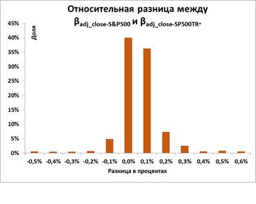
Rice. 3. The relative difference of the coefficients of β , calculated by regression of daily returns adj _ close on the index S & P 500 and SP 500 TR for 43 long-lived companies in 1988-2018.
At first glance, given the high sensitivity of the βi measurement results to the details of the methodology noted above, this coincidence may seem surprising. However, it seems natural to the authors, since each company makes a decision on the timing and amount of dividend payments independently. This means that the part of the market portfolio's return associated with the payment of dividends on the market portfolio should not correlate with the return of a single company, and therefore βi, evaluated on the two varieties of the s&P500 and SP500TR index should be the same.
A slightly larger difference is observed when comparing β i calculated in pairs: the yield on the close values and the s&P500 index and the yield on the adj_close values and the SP500TR index. In this case, the βi coefficients in 98% of the matched pairs differ by no more than 4%.
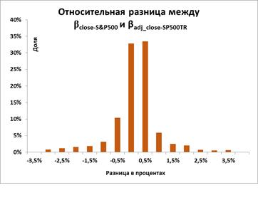
Rice. 4. The relative difference of the coefficients of β , calculated by regression of daily returns close on the index S & P 500 and adj _ close on the index SP 500 TR for 43 long-lived companies in 1988-2018.
When evaluating the beta companies included by Damodaran in the lists of industries considered in the article, using the Yahoo method (monthly data for a period of 3 years), the authors considered two options for regression of company returns calculated by prices adj _ closes the standard s&P500 index and the S&P500TR index.
However, the differences between the beta coefficients calculated by these two methods can be seen (see Yahoo sheets in files uploaded to the cloud [30], Betas _ Utility _( General )_2018. xlsm , Betas _ Retail _( Grocery _ and _ Food )_2018. xlsm , Betas _ Food _ Wholesalers _2018. xlsm , Betas _ Shoe _2018. xlsm , Betas _ Automotive _2018. xlsm .) are slightly higher than those shown in table 3 and figure 3.4. However, even in this case, for stable companies of different industries listed on the NYSE and NASDAQ stock exchanges, these differences are on average 1%-15% of the corresponding 95% confidence intervals of beta companies ' ratings.
Thus, all these differences are obviously not statistically significant for the typical values of error in estimating the beta coefficients.
Conclusion
The calculations of systematic risk coefficients β i based on empirical data on the returns of various companies and market portfolios show that the estimates βi provided by various«reliable providers » and obtained by analyzing data on the returns of the company and the market, selected for different periods of time in the past with different intervals between the moments of fixing stock prices and the index, differ very significantly. Most of these differences are probably due to statistical errors in the β i estimates, which in many cases may be comparable and sometimes exceed these estimates themselves (see table 2).
An analysis of the time dependencies of estimates of systematic risk coefficients β i(t) obtained over short (3-month and 2-year) sample periods shows that, apparently, most of the chaotic and undulating changes in coefficients βi for stable companies that have long been listed on Mature stock markets, is an artifact due to statistical errors in these estimates (Fig.2 a-d). Since "reliable providers", with the exception of Bloomberg, do not specify standard deviations of their "beta" I ratings, a conscientious researcher should treat them with caution.
As noted at the beginning of the article, the systematic risk ratio of a portfolio or industry (β P or βsector) is one of the Central elements of financial theory and is not entirely related to the theory of CAPM, although it is almost the only quantitative tool for estimating the required return on equity for companies from various sectors of the economy based on the systematic risk of the industry. In the end, the answer to the question: what kind of returns the market requires from industries with different coefficients of systematic risk, should give an analysis of the vast documented experience of financial markets. But, as the examples discussed in this article show, even the problem of "measuring" sector coefficients based on empirical data on the correlation of returns of companies that represent the industry and the market can hardly be considered solved.
In the following papers, the authors intend to consider whether the differences in the estimates of βi related to the choice of the interval between successive values of stock prices and the period on which the coefficient is evaluated β i, are completely random or do they have a systematic component? The answer to this question requires, in our opinion, both a large-scale empirical study of all companies listed on the Mature stock markets of the NYSE and NASDAQ, and a theoretical study of the properties of estimating the covariance and variance of returns of these companies and the market portfolio on samples with different periods and with different intervals between the moments of fixing returns.
References
1. Blume M. E. On the Assessment of Risk // Journal of Finance. — 1971. — Vol. 26. — No. 1. — pp. 1–10. — DOI: 10.2307/2325736.
2. Jensen M. Risk, the Pricing of Capital Assets, and the Evaluation of Investment Portfolios // The Journal of Business. — 1969. — Vol. 42. — No. 2. — pp. 167–247. — URL: https://www.empirical.net/wp-content/uploads/2012/04/Jensen1969.pdf.
3. Breili R., Maiers S. Printsipy korporativnykh finansov. Moskva: Olimp-Biznes, 2012. — 1008 s. — ISBN 978-5-9693-0089-7.
4. Timofeev D. V. Modelirovanie suverennoi premii za risk na razvivayushchikhsya rynkakh kapitala // Korporativnye finansy. — 2015. — №2 (34). — S. 54–72.
5. Sharp W. F. Capital Assets Prices: A Theory of Market Equilibrium under conditions of Risk // The Journal of Finance. — 1964. — Vol. 19. — No. 3. — pp. 425-42. — DOI: https://doi.org/10.1111/j.1540-6261.1964.tb02865.x.
6. Lintner J. The Valuation of Risk Assets and the Selection of Risky Investments in Stock Portfolios and Capital Budgets // The Review of Economics and Statistics. — 1965. — Vol. 47. — No. 1. — pp. 13–37. — URL: http://www.jstor.org/stable/1924119.
7. Shvedov A. C. Teoriya effektivnykh portfelei tsennykh bumag. Moskva: GU VShE, 1999. — 144 c. — ISBN 5-7598-0066-3.
8. Damodaran A. Investitsionnaya otsenka. Instrumenty i metody otsenki lyubykh aktivov. Moskva: Al'pina Pablisher, 2018. — 1316 s. — ISBN 978-5-9614-6650-8.
9. Fernandez P., Pershin V., Fernández Acín I. Discount Rate (Risk-Free Rate and Market Risk Premium) Used for 41 Countries in 2017: A Survey. // SSRN. — 2017 April 17. DOI: http://dx.doi.org/10.2139/ssrn.2954142.
10. Dranev Yu. Ya., Nurdinova Ya. S., Red'kin V. A., Fomkina S. A. Modeli otsenki zatrat na sobstvennyi kapital kompanii na razvivayushchikhsya rynkakh kapitala. // Korporativnye finansy. — 2012. — № 2 (22). — S. 107–117.
11. Graham J. R., Harvey C. R. The Equity Risk Premium in 2018 // SSRN. — 2018. — 21 p. — DOI: http://dx.doi.org/10.2139/ssrn.3151162.
12. Fama E. F., French K. R. A five-factor asset pricing model // Journal of Financial Economics. — 2015. — Vol. 116. Issue 1.— pp. 1–22. — DOI: https://doi.org/10.1016/j.jfineco.2014.10.010.
13. Fama E. F., French K. R. Dissecting anomalies with a five-factor model // Review of Financial Studies. — 2016. — Vol. 29. — pp. 69–103.
14. Fama E. F., French K. R. International tests of a five-factor asset pricing model // Journal of Financial Economics. — 2017. — Vol. 123. — Issue 3. — pp. 441–463. — DOI: https://doi.org/10.1016/j.jfineco.2016.11.004.
15. Cooper I., Maio P. F. Asset Growth, Profitability, and Investment Opportunities // Management Science. — 2018. — 47 p. — DOI: http://dx.doi.org/10.2139/ssrn.2554706.
16. Maio P. F., Silva A. C. Asset Pricing Implications of Money: New Evidence // SSRN. — 2018, Oct. 30. — 54 p. — DOI: http://dx.doi.org/10.2139/ssrn.2388879.
17. Hou K., Xue C., Zhang L. Digesting anomalies: an investment approach // Review of Financial Studies. — 2015. — Vol. 28. — pp. 650–705.
18. Wilcox R. R. Introduction to robust estimation and hypothesis testing. — 3rd edition. — Cambridge, Massachusetts (USA): Academic Press, 2012. — 608 p. — ISBN 9780123869838.
19. Amaya D., Christoffersen P., Jacobs K., Vasquez A. Does Realized Skewness Predict the Cross-Section of Equity Returns? // Journal of Financial Economics (JFE). — 2015 Mar 9. — 58 p. — DOI: http://dx.doi.org/10.2139/ssrn.1898735.
20. Akhmetshin E. M., Osadchy E. A. New requirements to the control of the maintenance of accounting records of the company in the conditions of the economic insecurity // International Business Management. — 2015. — No. 9. — Issue 5. — pp. 895–902. — DOI: 10.3923/ibm.2015.895.902.
21. Damodaran A. Estimating Risk Parameters // New York University, Leonard N. Stern School Finance Department Working Paper Series. — 1999. — 019.
22. Damodaran A. Equity Risk Premiums (ERP): Determinants, Estimation and Implications — The 2018 Edition. New York: Stern School of Business, 2018. — 133 p. — DOI: http://dx.doi.org/10.2139/ssrn.3140837.
23. Hamada R. S. The Effect of Firms Capital Structure on the Systematic Risk of Common Stocks // Journal of Finance. — 1972. — Vol. 27. — pp. 435–452.
24. Guseinov B. M. Problemy rascheta koeffitsienta beta pri otsenke stoimosti sobstvennogo kapitala metodom CAPM dlya rossiiskikh kompanii. // Finansovyi menedzhment. — 2009. — № 1. — S. 76–83.
25. Mandelbroad B. Variation of certain speculative prices // Journal of Business. — 1963. — Vol. 36. — No. 4. — pp. 394–419.
26. Fama E. F. The Behavior of Stock Market Prices // The Journal of Business. — 1965. — pp. 34–105.
27. Friedman B. M., Laibson D. I. Economic Application of Extraordinary Movements in Stock Prices // Brookings Papers on Economic Activity. — 1989. — Vol. 20. — No. 2. — pp. 137–189.
28. Piters E. Khaos i poryadok na rynkakh kapitala. Moskva: Mir, 2000. — 276 s. — ISBN 5-03-003356-4.
29. Fernandez P., Carelli J. P., Ortiz Pizarro A. The Market Portfolio is NOT Efficient: Evidences, Consequences and Easy to Avoid Errors // SSRN. — 2017 Oct 17. — 23 p. DOI: http://dx.doi.org/10.2139/ssrn.2741083.
30. Zaitsev M.G., Varyukhin S.E. Raschet koeffitsientov beta dlya kompanii iz pyati otraslei SShA. [Elektronnyi resurs]. — 2018. — URL: https://1drv.ms/f/s!ArFRI2i3V3yXjcVDQqLhBR1ufuidug. (Data obrashcheniya: 22.01.2019).
31. Damodaran, A. Damodaran Online. [Elektronnyi resurs]. — 2019. — URL: http://pages.stern.nyu.edu/~adamodar/ (Data obrashcheniya: 22. 01. 2019)
Link to this article
You can simply select and copy link from below text field.
|
|